| f(x) = | (x - a)(x - b) | / | (x - d)(x - e) |
| f(x) = | (x - a)(x - b) | / | (x - d)(x - e) |
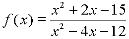
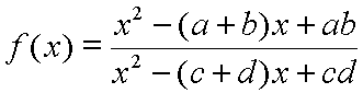
| f(x) = | x2 + c1nx + c0n | / | x2 + c1dx + c0d |
x:
y:
Below is a program which demonstrates the behavior of a rational function. The type of rational function which it demonstrates is a second degree polynomial divided by a second degree polynomial, that is, a quadratic divided by a quadratic. Right below the program is a link to an explanation of how to use it. All of that is followed by a detailed discussion of the program and of rational function behavior in general.
This program graphs this function:
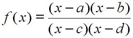
| f(x) = | (x - a)(x - b) | / | (x - d)(x - e) |
| f(x) = | (x - a)(x - b) | / | (x - d)(x - e) |
| f(x) = | x2 + c1nx + c0n | / | x2 + c1dx + c0d |
This is a link to instructions about this program and other similar programs in this rational function section. Quick instructions for the above program are directly below:
Detailed explanation of the program and rational function behavior in general
![]() Roots
Roots
Again, this graphing program presents the graphs of rational functions which are second degree polynomials divided by second degree polynomials. An example of such a rational function would be:
You need to visualize this rational function with the polynomials in factored form. That is, the above function, f(x), would need to be seen as:
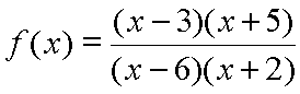
When investigating rational functions, the first move is usually to factor the polynomials like above. You factor both polynomials to find their roots. In the above example the roots of the numerator are:
roots of the numerator: x = 3 and x = -5
And the roots of the denominator are:
roots of the denominator: x = 6 and x = -2
In the above program, the variables a and b are the roots of the numerator, and c and d are the roots of the denominator. So, you should imagine rational functions of this form:
If you were to multiply the above factors in the numerator and denominator, you would get a function that looked like this:
This last rational function might look a bit more normal than its factored version if one is thinking about the division of two polynomials, since polynomials are most often viewed in standard form. However, the roots of the polynomials are at the heart of this discussion, and finding them is the first step in analyzing a rational function.
| To understand rational functions it is important to understand the roots of the polynomials that make up the rational function. |
![]() Discontinuities
Discontinuities
Now, one can not divide by zero, so, when the polynomial in the denominator is equal to zero, the rational function is undefined. That is, there may be certain input values for x that cause the polynomial function in the denominator to output a zero. Consider, again, this function:
And, to clearly see the roots, perhaps it is better to view the function like this:
If x = 6, then the value of the denominator is zero since (x - 6) becomes (6 - 6), which is zero, and zero times the other factor, stated as (x + 2) or (x - (-2)), but now valued at (6 + 2) = 8, is zero. That is, zero times 8 is zero.
The function is undefined at x = 6 because you can not divide by 0.
For similar reasons the function will be undefined at x = -2. This value for x also makes the denominator equal to zero.
At the places where the function is undefined we say that the function is discontinuous. And we say that there are discontinuities in the function at the x-coordinates where it is undefined. Therefore, in the above function there are discontinuities at x = 6 and at x = -2.
| Discontinuities are locations for x values that make the function undefined. |
![]() Asymptotes
Asymptotes
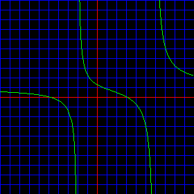
These discontinuities at x = 6 and at x = -2 show up on the graph as vertical asymptotes. Not all discontinuities in rational functions create vertical asymptotes, but these do. Some discontinuities are not asymptotic, but are removable. More about that later.
Vertical asymptotes show up as vertical white lines on the above applet. To plug the above function into the graphing applet you must set a, b, c, and d to the following values:
a = 3 |
b = -5 |
c = 6 |
d = -2 |
That is, make the roots of the quadratic in the numerator equal to 3 and -5, and make the roots in the denominator equal to 6 and -2. Go ahead and try that. It should look like the following picture. (Do not check the "Numerator" nor "Denominator" checkbox.)
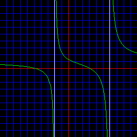
Notice that the above graph shows a vertical asymptote at x = 6. (Remember, the red lines are the x- and y-axes. Each blue line is an increment of 1.) There is also a vertical asymptote at x = -2, but let us concentrate on the one at x = 6 for the moment.
The function is undefined at x = 6 because that input value makes the denominator of the function equal to 0. To the immediate left of 6 the function outputs very large negative numbers making the graph of the function drop very steeply. We could prove this behavior by finding the value of the function with an input value a tiny bit to the left of x = 6. Moving over by 0.001 usually works fine. So, let us find the output value for x = 5.999:
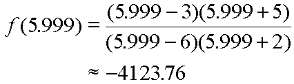
Clearly, to the immediate left of the asymptote the function takes on an output value much more negative than can be seen on the above picture. The above graph only goes to -10 along the y-axis.
Let us see what is happening to the immediate right of the vertical asymptote at x = 6. Again, we will step over by the tiny step of 0.001. This would create an input value of 6.001. Here is the output calculation:
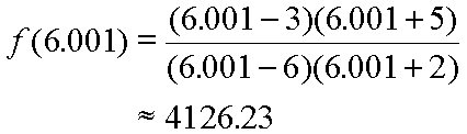
Well, it certainly looks like the function takes on very large positive values to the immediate right of x = 6. This behavior, large negative output to the left of x = 6 and large positive output to the right of x = 6, is what causes the asymptotic shape of the function at x = 6.
It is important to remember that the vertical asymptote is not a line that is part of the graph of the function. For this reason the asymptote is drawn in a different color. It is white, the actual function is green. The white asymptote line is a visual convenience in the diagram to show a line that the function approaches, but never touches. It is a good idea to see the graph of the function without this aid. The only problem with that is that often asymptotic behavior is not completely drawn to the edges of the diagram by computers. Ultimately, this is due to the fact that the computer diagram is made up of tiny discrete dots, called pixels, while the x, y real number plane is continuous. All the same, un-check the "Asymptotes" checkbox. It should look like this:
| Discontinuities may be asymptotic. |
![]() Discontinuities and the denominator polynomial
Discontinuities and the denominator polynomial
As we have seen this function has two discontinuities at the roots of the polynomial in the denominator, x = 6 and at x = -2. Now, the denominator is a second degree polynomial, often called a quadratic polynomial. A second degree polynomial graphs as a parabola. So, if we could see the graph of the denominator polynomial, we would see a graph of a parabola. Where that parabola crosses the x-axis locates the roots, or zeroes, of that parabola. These, of course, are the locations of the asymptotic discontinuities which we have been discussing. To see both the denominator parabola and the rational function graphed together check the 'Denominator' checkbox. It might be useful to have the asymptotes turned on, also. Try that. Here is a diagram that shows what it should look like, along with an explanatory note:
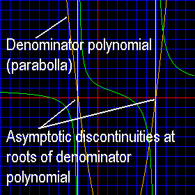
| Discontinuities are located at the roots of the denominator polynomial. |
![]() X-intercepts
X-intercepts
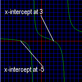
This function crosses the x-axis at two points. These points are called its x-intercepts. Simply put, an x-intercept will exist where the y, or output, value of the function equals zero. Now, the function we consider here is a rational function, so, since it is a division of polynomials, it may be considered a fraction. A fraction will be equal to zero only when its numerator is equal to zero. The numerator will be equal to zero at the roots of the polynomial in the numerator. The roots of the numerator polynomial are x = 3 and x = -5, as another quick look at our rational function in factored form will reveal:
So the x-intercepts should be at x = 3 and x = -5, since these make the y, or output, value of the function equal to zero. Another look at our current graph will demonstrate this:
| X-intercepts are where y =0 (and the function is defined). |
![]() X-intercepts and the numerator polynomial
X-intercepts and the numerator polynomial
The numerator polynomial graphs as a parabola, since it is of second degree. The roots of this parabola are the values which make the numerator of the rational function equal to zero, as explained above. On the program above if you check the 'Numerator' checkbox, then the numerator polynomial will be drawn along with the rational function. You should see that the roots of this parabola are the x-intercepts discussed directly above. Try that. Probably best seen with the asymptotes turned off, it should look like the following:
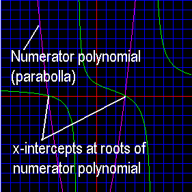
| The roots of the numerator polynomial are the x-intercepts (if the function is defined there). |
![]() Y-intercept
Y-intercept
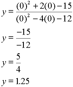
The y-intercept of a function occurs at the point where the function line crosses the y-axis. This would be where x = 0. So, if you set x equal to zero in the rational function, the function will output a value equal to the y-intercept. This is actually quite easy to do for rational functions. Since both the numerator and the denominator are polynomials in x, every term except the last constant term, (if present), in each polynomial becomes equal to zero. So, the value for the y-intercept is simply the ratio of the two last constant terms. This is easier to see than to explain. Here is our function again:
Or, expressed in 'y =' form:
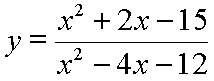
Now, to find the y-intercept plug in x = 0 and solve:
Again, let us look at our graph. Notice that it crosses the y-axis at y = 1.25:
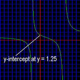
| The y-intercept is the ratio of the two last constant terms of the numerator and denominator polynomials. |
![]() End behavior model function
End behavior model function
A rational function is said to have an end behavior model function. The behavior of the end behavior model function and the behavior of the rational function are the same at large positive and large negative values of x.
In other words, the rational function and the end behavior model function act the same way as they each 'head out' to distant left and right values along the x-axis.
The end behavior model function, which we will here name m(x), is found by dividing the leading term of the numerator polynomial by the leading term of the denominator polynomial. One, of course, must view the rational function with the polynomials in standard form, not factored form. Here is another look at our function, polynomials in standard form:
For the function considered here the leading term of the numerator is x2, and the leading term of the denominator is also x2. The division of these two, as described above, yields the end behavior model function, m(x), as shown by:
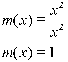
Or, if you want to consider this end behavior model function in 'y =' form, it would look like:
![]()
This, of course, is a horizontal line that crosses the y-axis at y = 1. That means that our rational function will approach this horizontal line for large positive and large negative input, or x, values. Although the graph on the applet above does not go far enough to the left or right to see this perfectly, one can see this end behavior fairly clearly. Below is our current graph with the end behavior model function drawn in as a white line:
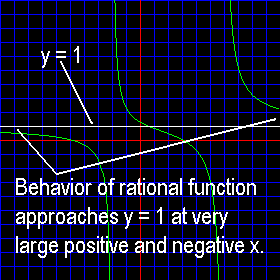
You should notice that for the rational functions which are presented with this applet the only possible end behavior model is m(x) = 1, since the division of the leading terms of the polynomials in the numerator and denominator will always be x2 / x2.
| The end behavior model function demonstrates the behavior of the rational function at extreme values for x. |
![]() Discontinuities which are not asymptotes
Discontinuities which are not asymptotes
Go to the program and set up the following situation. Be sure to notice that the only difference is that now x = 6 is a root of both the numerator and the denominator:
a = 6 |
b = -5 |
c = 6 |
d = -2 |
The graph should now look like this:
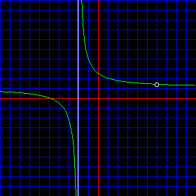
Notice that there used to be an asymptote at x = 6, but now there is not. (The asymptote at x = -2 is still there. We are not discussing that here.)
There is still a discontinuity at x = 6, that is, the function is still not defined at there because this value for x still makes the denominator equal to zero. And still if one were to imagine drawing the function line carefully, one would have to break the function line by picking up one's pen at x = 6. That break is represented on the graph by the little white circle.
However, this other type of discontinuity is not asymptotic, it is termed removable. We say that there is a removable discontinuity at x = 6.
The discontinuity at x = 6 is called removable because it can be removed, (or 'plugged'), simply by redefining the function at this point. That is, we could assign a certain value to the output, any value, really, at x = 6. A piecewise-definition of the function would work fine, such as:
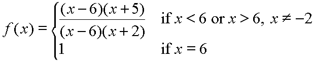
Notice that all we did was use the normal definition of our rational function for all values of x except x = 6, and, of course x = -2, which is our asymptotic discontinuity. Then we gave an output value of 1 to the function when x = 6. To remove the discontinuity it is not necessary to 'plug' the hole in the function line. One simply must provide an output value for the function for the value of x that causes the removable discontinuity. There is, of course, an actual (x, y) point on the real number plane that would 'plug' the hole, and, perhaps, in some applications one would want to know it and use it in a similar piecewise-definition for the function. Finding that point is a calculus problem.
Lastly, let us notice something about x-intercepts with this version of our rational function. Suppose we did not redefine the function so as to remove the discontinuity at x = 6. Then we are back to the function in this form:
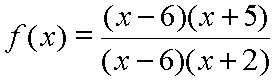
It may look at first glance that there should be an x-intercept at x = 6 because this value makes the numerator equal to zero, which makes the output, or y, value equal to zero, and that is what we mean by an x-intercept. Except the function can not have an x-intercept at x = 6 because it is not defined there. It is discontinuous, (with a removable discontinuity), at x = 6.
| Removable (and not asymptotic) discontinuities form when the numerator and denominator polynomials share common roots. |
![]() Conclusion
Conclusion
Well, if you got this far, you gone through most of what you need to know to understand rational functions of many types, not just second degree polynomials divided by second degree polynomials. For example, this same reasoning would be used in an investigation of a first degree polynomial divided by a third degree polynomial.
Go back to the program and play with it. Try out several combinations of for roots both in the numerator and denominator. Adjust it till you understand how to generate asymptotic and removable discontinuities. And, of course, go on to explore the other topics about rational functions in Zona Land.
| Play with the program. |
![]() P. S., So why is
this called the simple version?
P. S., So why is
this called the simple version?
Perhaps you remember that the link from the rational functions home page labeled this 'Simple 2nd Degree / 2nd Degree'. Well, observant mathematicians will notice that this applet will not graph every type of rational function that is a second degree polynomial divided by a second degree polynomial. It only demonstrates those in which the leading coefficient is equal to one in both the numerator and the denominator. For example, you could not study this rational function with this applet:
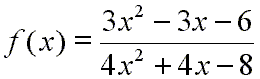
This function factors like so:
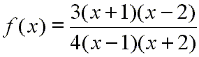
The program here provides no way to enter the factor of 3 in the numerator nor the factor of 4 in the denominator. However, the behavior of such functions as this one can be understood using the same methods described here. In fact, the behavior of most rational functions can be understood with these methods. As one closing note, see that the end behavior model function for the rational function above is not y = 1, but:
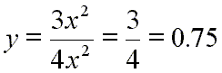
The end behavior model function is still a horizontal line. This is really the only difference one would need to consider in understanding this type of second degree polynomial over second degree polynomial rational function. Rational functions of this more general type will be demonstrated in other obvious sections in the Rational Functions Department of the Function Institute.
| The information here is applicable to all types of rational functions. |