Definition of a Rational Function

A rational function is basically a division of two polynomial functions. That is, it is a polynomial divided by another polynomial. In formal notation, a rational function would be symbolized like this:

Where s(x) and t(x) are polynomial functions, and t(x) can not equal zero.

An Example

Here is an example of a rational function:

To understand the behavior of a rational function it is very useful to see its polynomials in factored form. The polynomials in the numerator and the denominator of the above function would factor like this:

The Domain

Now the roots of the denominator are obviously x = -3 and x = 6. That is, if x takes on either of these two values, the denominator becomes equal to zero. Since one can not divide by zero, the function is not defined for these two values of x. We say that the function is discontinuous at x = -3 and x = 6.

Other values for x do not cause the function to become undefined, so, we say that the function is continuous at all other values for x. In other words, all real numbers except -3 and 6 are allowed as inputs to this function. The domain for the function, therefore, as expressed in interval notation is:

The x-intercepts

The x-intercepts for this function would be where the output, or y-value, equals zero. A rational function can be considered a fraction, and a fraction is equal to zero when the numerator is equal to zero. For our rational function example this happens when the polynomial in the numerator is equal to zero, and this will happen at the roots of this polynomial. The roots of the numerator polynomial are x = -5 and x = 4. That is, when x takes on either of these two values the numerator becomes zero, and the output of the function, or y-value, also becomes zero.

So, the x-intercepts for this rational function are x = -5 and x = 4. Notice that the function is defined at these two values. (It is only not defined at x = -3 and x = 6.) That makes these true x-intercepts. If the function was not defined at x = 4 because 4 was a root of the denominator polynomial, (which it is not in our example here), then x = 4 would not be an x-intercept even though it made the numerator equal to zero. One can not have an x-intercept for a function at a point where the function does not exist!

The y-intercept

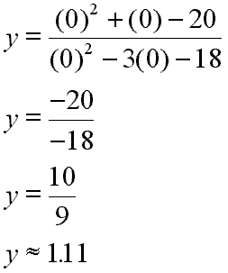
What about the y-intercept? Well, they occur where the input, or x, value equals zero. If we look at our first un-factored form for this function, expressed in 'y =' form, we have:

Now, setting x = 0 we get:

That is, the graph crosses the y-axis at y = 10/9 (about 1.11). Notice that when you express the polynomials of a rational function in standard form, then the y-intercept is simply the ratio of the final terms for the two polynomials.

The Graph

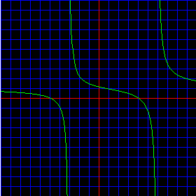
Let us look at a graph of this function:

The red lines are the x- and y-axes; the blue grid marks off unit distances; the green line is the function. Realize the following:

• The function line is discontinuous, or 'breaks', at x = -3 and x = 6. That is, if you were drawing the graph by hand, you would have to lift the pen off the paper at at x = -3 and x = 6. That is what we mean by a discontinuity. Notice that these locations for the discontinuities, (x = -3 and x = 6), are the same as we reasoned above. That is, x = -3 and x = 6 are the roots of the polynomial in the denominator.
• The function crosses the x-axis at x = -5 and x = 4. These are the same as the values which we calculated above for the x-intercepts.
• The function crosses the y-axis just a bit above 1, at about 1.1. This is the same location as the calculated y-intercept above.

The End Behavior Model Function

The way that a function is shaped when the input, or x, is very large positively or very large negatively is called its end behavior. That is, the end behavior of a function describes how it acts as x approaches positive and negative infinity. One might say that the end behavior of a function is described by how it 'heads out' to the right and left on the graph far away from the origin.

In the graph above notice how the graph is leveling off to a height of about y = 1 as x gets large positively or negatively. That is, at the left and right edge of the graph the function starts to act like the function described as:

This function, y = 1, is called the end behavior model function for the rational function on the graph. You can find it without drawing the graph by dividing the leading term of the polynomial in the numerator by the leading term of the polynomial in the denominator. Our function under consideration is this:

The leading term of the polynomial in the numerator is:

The leading term of the polynomial in the denominator is:

The division of these two leading terms, numerator leading term over denominator leading term, is:

And, of course, this makes the following end behavior model function:

The Range

An examination of the graph above will indicate that all real numbers are available for output. The left most fork of the graph looks like it will rise not quite to y = 1, and the right most fork looks like it may not quite drop to y = 1; so, one might at first suggest that y = 1 is not in the range. However, if you examine the central portion of the graph, you can see that y = 1 is definitely a member of the range. So, all real numbers are present in the range. In interval notation the range would look like this:

Summary

This has been an introduction to rational functions and their behaviors. For more details and examples, examine the other topics in the rational function section of the Function Institute. The link labeled 'Simple 2nd Degree / 2nd Degree' goes over the material presented here in much more detail and contains an animated Java applet rational function graphing utility, for example.